


When working with well log data, one of the first things you want to know isn’t what the data looks like, it’s whether the data is even there.
In my previous article, I looked at how lasio and rich can be used together to inspect LAS file metadata in the terminal: curve names, units, descriptions, and basic completeness.
That approach works well for answering “what’s in this file?”
But there’s a related question that’s harder to answer from a table alone:
Where is the data, and where isn’t it?
A curve might show 85% completeness overall, but if the missing 15% happens to sit right across your reservoir interval, that number is misleading. What you really want is a spatial view of availability, i.e. something that shows you which curves have data at which depths.
This article builds on the previous one by creating a simple terminal-based coverage heatmap. A coloured grid in the terminal that makes data gaps obvious at a glance.
The problem with summary statistics alone
When you call .isna().mean() on a DataFrame, you get a single number per curve. That’s useful, but it hides the distribution of missing data.
Consider two curves, both with 80% completeness:
One has data across the full logged interval with scattered nulls throughout
The other has a solid block of data in the upper section and nothing below a certain depth
Both report the same percentage. But in practice, they tell very different stories about what you can do with that data.
This is especially common with LAS files that have been spliced from multiple logging runs or contain a mix of open-hole, cased-hole, and derived curves. The coverage pattern matters as much as the coverage number.
What would help is a way to see, at a glance, which curves have data and where that data is without leaving the terminal.
Binning depth into rows
The basic idea behind the heatmap is straightforward: divide the depth range into a fixed number of bins, and for each bin, check whether each curve has any valid data in that interval.
This gives you a grid where each row is a depth range and each column is a curve. If the curve has at least one non-null value in that bin, it gets marked as having data. Otherwise, it’s empty.
The number of bins controls how much detail you see:
Too few and you lose resolution.
Too many and the terminal output becomes unwieldy.
Somewhere around 50 rows tends to work well for most files.
import numpy as np
import pandas as pd
import lasio

las = lasio.read(”L05-15-Spliced.las”)
df = las.df()

depth = df.index.to_numpy()
dmin, dmax = float(depth.min()), float(depth.max())

rows = 50
edges = np.linspace(dmin, dmax, rows + 1)
The edges array defines the boundaries between bins. For 50 rows, you get 51 edges, one for each boundary.
Checking coverage per bin
For each bin, we need to know whether each curve has any valid data in that depth range. This is a simple mask-and-check operation:
curves = [”GR”, “CAL”, “CN”, “ZDEN”, “ZDNC”, “PORZ”, “MPHS”, “MPHE”]

# Filter to curves that actually exist in the file
curves = [c for c in curves if c in df.columns]

cov = np.zeros((rows, len(curves)), dtype=bool)

for i in range(rows):
    lo, hi = edges[i], edges[i + 1]
    if i < rows - 1:
        mask = (depth >= lo) & (depth < hi)
    else:
        mask = (depth >= lo) & (depth <= hi)

    band = df.loc[mask, curves]
    if len(band) > 0:
        cov[i, :] = band.notna().any(axis=0).to_numpy()
The result is a boolean matrix: True where data exists, False where it doesn’t.
The last bin uses <= instead of < for the upper boundary to ensure the final depth sample isn’t excluded. It’s a small detail, but one that avoids a subtle off-by-one issue at the bottom of the file.
Rendering the heatmap with rich
This is where rich earns its keep. We take that boolean matrix and render it as a coloured table in the terminal.
from rich.console import Console
from rich.table import Table
from rich.text import Text

console = Console(width=200)

table = Table(
    title=”LAS Data Coverage Heatmap”,
    show_header=True,
    header_style=”bold”,
    show_lines=False,
    padding=(0, 1),
)

depth_unit = las.well.STRT.unit or “”
unit_label = f” ({depth_unit})” if depth_unit else “”

table.add_column(f”Depth{unit_label}”, style=”cyan”, no_wrap=True)
for c in curves:
    table.add_column(c, justify=”center”, no_wrap=True)

cell = “    “

for i in range(rows):
    depth_label = f”{edges[i]:.0f}”
    row_cells = []
    for j in range(len(curves)):
        if cov[i, j]:
            row_cells.append(Text(cell, style=”on green”))
        else:
            row_cells.append(Text(cell))
    table.add_row(depth_label, *row_cells)

table.add_row(f”{edges[-1]:.0f}”, *[Text(”“) for _ in curves])

console.print(table)
console.print(
    Text(”  Legend: “, style=”bold”)
    + Text(” data “, style=”on green”)
    + Text(”  blank = no data”, style=”dim”)
)
Each cell is a small block of coloured text. Green means there’s data in that depth bin for that curve. Blank means there isn’t. The result is a compact visual grid you can scan in a second or two.
The cell = " " line might look odd , it’s just four spaces that give each cell enough width to be visible. Without it, the table cells would be too narrow for the background colour to register.
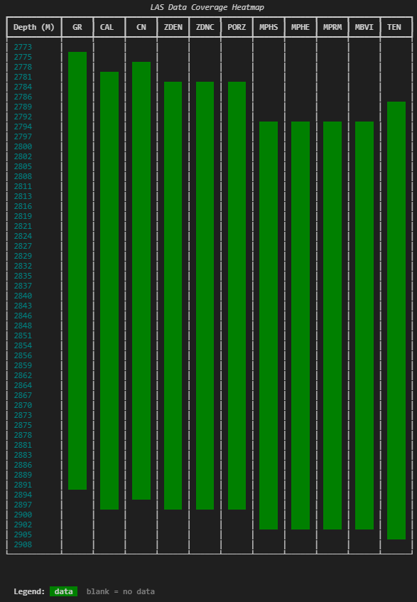
What you get is something that immediately shows you the shape of your data. You can see where logging starts and stops for each curve, where there are gaps, and which curves share the same coverage pattern.
Finding and reporting gaps
The heatmap gives you the visual picture, but it helps to have the specifics as well. A companion summary table can report the exact start and stop depths for each curve, the overall coverage percentage, and the locations of any significant gaps.
A gap here means a contiguous run of null values within the curve’s data range. Short runs of one or two samples are ignored , those are normal and not usually worth flagging. The threshold used below is three or more consecutive samples.
def find_gaps(depth_index, series, min_gap_samples=3):
    valid = series.notna().to_numpy()
    if not valid.any():
        return None, None, []

    depths = depth_index.to_numpy()
    valid_depths = depths[valid]
    start = float(valid_depths[0])
    stop = float(valid_depths[-1])

    in_range = (depths >= start) & (depths <= stop)
    mask = ~valid & in_range

    gaps = []
    i = 0
    n = len(mask)
    while i < n:
        if mask[i]:
            j = i
            while j < n and mask[j]:
                j += 1
            if (j - i) >= min_gap_samples:
                gaps.append((float(depths[i]), float(depths[j - 1])))
            i = j
        else:
            i += 1

    return start, stop, gaps
The logic walks through the depth index, looking for runs of nulls that fall within the curve’s valid data range. It ignores anything before the first valid sample or after the last , those aren’t gaps, they’re just where the curve starts and stops.
This function returns three things: where the curve starts, where it stops, and a list of any interior gaps longer than the threshold.
Putting the summary together
With the gap information in hand, we can build a second rich table that gives you the numbers behind the heatmap:
dfi = df[curves].sort_index()

summary = Table(
    title=”Curve Coverage Summary”,
    show_header=True,
    header_style=”bold”,
)
summary.add_column(”Curve”, style=”cyan”, no_wrap=True)
summary.add_column(f”Start{unit_label}”, justify=”right”)
summary.add_column(f”Stop{unit_label}”, justify=”right”)
summary.add_column(”Coverage”, justify=”right”)
summary.add_column(”Gaps”, no_wrap=False)

for c in curves:
    start, stop, gaps = find_gaps(dfi.index, dfi[c])
    total_valid = int(dfi[c].notna().sum())
    total_samples = len(dfi)
    coverage_pct = (total_valid / total_samples * 100) if total_samples else 0

    if start is None:
        summary.add_row(c, “-”, “-”, “0%”, “[red]No data[/red]”)
        continue

    gap_text = (
        “, “.join(f”{top:.1f}-{bot:.1f}” for top, bot in gaps)
        if gaps
        else “[green]None[/green]”
    )

    summary.add_row(
        c,
        f”{start:.1f}”,
        f”{stop:.1f}”,
        f”{coverage_pct:.0f}%”,
        gap_text,
    )

console.print(summary)
This pairs well with the heatmap. The heatmap shows you the shape of the problem. The summary gives you the specifics: exact depths, exact coverage percentages, exact gap locations.
Together, they answer most of the questions you’d typically need a log plot or a notebook to resolve.
Wrapping it into a reusable function
In practice, you probably don’t want to copy this code every time you open a new file. The full version wraps everything : the binning, the heatmap, the gap detection, and the summary into a single function:
coverage_heatmap(df, curves=[”GR”, “CAL”, “CN”, “ZDEN”], rows=50, depth_unit=”M”)You pass it a DataFrame, optionally specify which curves to include, how many depth bins you want, and the depth unit for labelling. It handles the rest.
If you don’t specify curves, it defaults to showing everything in the DataFrame. In practice, picking a manageable subset of key curves tends to give you a clearer picture than showing all 30+ columns at once.
The full code is available at the end of this article.
Why this belongs in your workflow
This kind of output doesn’t replace log plots or statistical analysis. But it occupies a useful gap between loading a file and starting interpretation.
In the few seconds it takes to run, you get answers to questions that would otherwise take longer to surface:
Does this curve actually have data across the interval I care about?
Are there gaps I need to deal with before splicing or merging?
Which curves share the same coverage pattern, and which don’t?
Is that “85% complete” curve actually missing data right where it matters?
These are the kinds of things that, if you don’t check explicitly, tend to show up later as confusing plot behaviour or unexpected nulls in a calculation.
And that’s the same theme from the previous article: inspect first, decide deliberately, then move on.
The tools don’t need to be complex. They just need to make the state of the data obvious.
Full code
The complete script, including the coverage_heatmap function and the find_gaps helper, is below. It reads a LAS file, selects a subset of key curves, and renders both the heatmap and summary table in the terminal.
import numpy as np
import pandas as pd
import lasio
from rich.console import Console
from rich.table import Table
from rich.text import Text

console = Console(width=200)

las = lasio.read(”L05-15-Spliced.las”)
df = las.df()


def find_gaps(depth_index, series, min_gap_samples=3):
    “”“Find data start, stop, and gaps for a single curve.”“”
    valid = series.notna().to_numpy()
    if not valid.any():
        return None, None, []

    depths = depth_index.to_numpy()
    valid_depths = depths[valid]
    start = float(valid_depths[0])
    stop = float(valid_depths[-1])

    in_range = (depths >= start) & (depths <= stop)
    mask = ~valid & in_range

    gaps = []
    i = 0
    n = len(mask)
    while i < n:
        if mask[i]:
            j = i
            while j < n and mask[j]:
                j += 1
            if (j - i) >= min_gap_samples:
                gaps.append((float(depths[i]), float(depths[j - 1])))
            i = j
        else:
            i += 1

    return start, stop, gaps


def coverage_heatmap(df, curves=None, rows=60, depth_unit=”“):
    “”“Render a terminal coverage heatmap with a per-curve gap summary.”“”
    if curves is None:
        curves = list(df.columns)
    if not curves:
        console.print(”[red]No matching curves found.[/red]”)
        return

    dfi = df[curves].sort_index()
    depth = dfi.index.to_numpy()
    dmin, dmax = float(depth.min()), float(depth.max())
    edges = np.linspace(dmin, dmax, rows + 1)

    # Binary coverage per bin
    cov = np.zeros((rows, len(curves)), dtype=bool)
    for i in range(rows):
        lo, hi = edges[i], edges[i + 1]
        if i < rows - 1:
            m = (depth >= lo) & (depth < hi)
        else:
            m = (depth >= lo) & (depth <= hi)
        band = dfi.loc[m, curves]
        if len(band) > 0:
            cov[i, :] = band.notna().any(axis=0).to_numpy()

    # Per-curve stats
    curve_stats = {}
    for c in curves:
        start, stop, gaps = find_gaps(dfi.index, dfi[c])
        total_valid = int(dfi[c].notna().sum())
        total_samples = len(dfi)
        curve_stats[c] = {
            “start”: start,
            “stop”: stop,
            “gaps”: gaps,
            “coverage_pct”: (
                total_valid / total_samples * 100
            ) if total_samples else 0,
        }

    # Heatmap table
    unit = f” ({depth_unit})” if depth_unit else “”
    table = Table(
        title=”LAS Data Coverage Heatmap”,
        show_header=True,
        header_style=”bold”,
        show_lines=False,
        padding=(0, 1),
    )
    table.add_column(f”Depth{unit}”, style=”cyan”, no_wrap=True)
    for c in curves:
        table.add_column(c, justify=”center”, no_wrap=True)

    cell = “    “
    for i in range(rows):
        depth_label = f”{edges[i]:.0f}”
        row_cells = []
        for j in range(len(curves)):
            if cov[i, j]:
                row_cells.append(Text(cell, style=”on green”))
            else:
                row_cells.append(Text(cell))
        table.add_row(depth_label, *row_cells)

    table.add_row(f”{edges[-1]:.0f}”, *[Text(”“) for _ in curves])
    console.print(table)
    console.print(
        Text(”  Legend: “, style=”bold”)
        + Text(” data “, style=”on green”)
        + Text(”  blank = no data”, style=”dim”)
    )

    # Summary table
    console.print()
    summary = Table(
        title=”Curve Coverage Summary”,
        show_header=True,
        header_style=”bold”,
    )
    summary.add_column(”Curve”, style=”cyan”, no_wrap=True)
    summary.add_column(f”Start{unit}”, justify=”right”)
    summary.add_column(f”Stop{unit}”, justify=”right”)
    summary.add_column(”Coverage”, justify=”right”)
    summary.add_column(”Gaps”, no_wrap=False)

    for c in curves:
        s = curve_stats[c]
        if s[”start”] is None:
            summary.add_row(c, “-”, “-”, “0%”, “[red]No data[/red]”)
            continue

        gap_text = (
            “, “.join(f”{top:.1f}-{bot:.1f}” for top, bot in s[”gaps”])
            if s[”gaps”]
            else “[green]None[/green]”
        )
        summary.add_row(
            c,
            f”{s[’start’]:.1f}”,
            f”{s[’stop’]:.1f}”,
            f”{s[’coverage_pct’]:.0f}%”,
            gap_text,
        )

    console.print(summary)


# Select key curves
key_curves = [
    “GR”, “CAL”, “CN”, “ZDEN”, “ZDNC”,
    “PORZ”, “MPHS”, “MPHE”, “MPRM”, “MBVI”, “TEN”
]
available = [c for c in key_curves if c in df.columns]

if not available:
    available = list(df.columns)

depth_unit = las.well.STRT.unit or “”
coverage_heatmap(df, curves=available, rows=50, depth_unit=depth_unit)