


In my last article I built a raincloud plot from scratch in matplotlib. This was a combination of a half-violin for the shape (cloud), the raw points jittered underneath (the rain), and a boxplot at the bottom giving a summary of the data distribution.
Even though we can build the plot by hand (and as usual) there is a dedicated library which wraps most of that up. This allows you to write fewer lines of code to achive what you are looking for.
ptitprince is the Python port of the original RainCloudPlots project that introduced the chart, and it sits on top of seaborn.
Setup and data
First, we need to install the library from PyPI:
pip install ptitprinceFor the data, we are using a synthetic dataset representing porosity for four geological formations, built to show different distributions we may expect in the subsurface.
Formation A is bimodal, the sort of split you get when a sand and an interbedded shale share a zone. B is tight and unimodal, C is right-skewed, and D has only eighteen samples.
import numpy as np
import pandas as pd
import matplotlib.pyplot as plt
import ptitprince as pt

rng = np.random.default_rng(42)

n = 300
form_a = np.concatenate([rng.normal(0.10, 0.015, n // 2),
                         rng.normal(0.22, 0.020, n // 2)])   # bimodal: sand/shale mix
form_b = rng.normal(0.18, 0.012, n)                          # tight, unimodal
form_c = 0.06 + rng.gamma(2.0, 0.018, n)                     # right-skewed
form_d = rng.normal(0.15, 0.020, 18)                         # very small sample

data = pd.DataFrame({
    "formation": (["A"] * len(form_a) + ["B"] * len(form_b)
                  + ["C"] * len(form_c) + ["D"] * len(form_d)),
    "porosity": np.concatenate([form_a, form_b, form_c, form_d]),
})
Generating the Basic Raincloud Plot
The library’s main entry point is RainCloud, and the basic call looks similar to how seaborn calls plots.
fig, ax = plt.subplots(figsize=(8, 5))
pt.RainCloud(x="formation", y="porosity", data=data, orient="h", ax=ax)
ax.set_xlabel("Porosity (frac)")
ax.set_ylabel("Formation")
Once we run the above code, we get back the following chart.
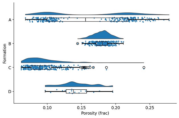
The default raincloud output from ptitprince.
With essentially all three layers are there for each formation, we can gain a good understanding of our data very quickly.
Compared with the thirty-odd lines of the hand-built version, that is a real saving.
The defaults are not perfect and almost looks like a basic matplotlib plot. Nothing wrong with that, but if you have followed my previous articles you can see how much I enjoy transforming matplotlib figures into something much better looking.
In this case, the boxplot sits directly on top of the rain, so the box hides some of the points it is meant to summarise, and the outlier fliers on the box duplicate points that are already visible in the rain. The layers are all present, but they are all fighting for the same space.
Tidying Up the Raincloud Plot
Customisation in ptitprince works in two ways.
A handful of top-level parameters control the layout, and everything else passes through to the underlying seaborn calls using prefixed keyword arguments: anything starting cloud_ goes to the half-violin, box_ to the boxplot, rain_ to the strip plot, and point_ to the optional mean marker.
The single most useful parameter I have found to tidy up the overlapping boxplot is move This shifts the rain (points) downwards and away from the box:
fig, ax = plt.subplots(figsize=(8, 5))
pt.RainCloud(
    x="formation", y="porosity", data=data, orient="h", ax=ax,
    move=0.2,                 # shift the rain clear of the box
    width_viol=0.7,           # cloud width
    point_size=3,             # rain marker size
    alpha=0.6,                # transparency for cloud and rain
    box_showfliers=False,     # outliers already visible in the rain
)
ax.set_xlabel("Porosity (frac)")
ax.set_ylabel("Formation")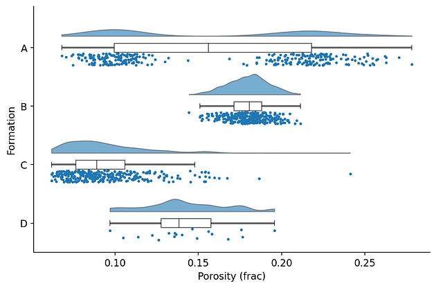
Tidied up version of the rain cloud plots with the rain sittin clear of the box, no fliers and no competing or overlapping elements.
By changing a few extra arguments we can make the chart tidier and easier to read.
Each layer now has it’s own space, the duplicated outliers are gone, and the transparency lets dense regions of rain show as darker bands. This is enough for making something quickly to help with the analysis.
Making it publication ready
For a figure going into a report or a paper, the tidied version still needs the usual finishing work: consistent colours, axis labels with units, sample counts, a title, and gridlines.
There are two ways we can get there.
The first is the prefixed kwargs handle anything that belongs to a layer, and the second, is by adding standard matplotlib calls because RainCloud draws onto an ordinary matplotlib Axes.
formations = ["A", "B", "C", "D"]
colours = ["#4C72B0", "#55A868", "#C44E52", "#8172B3"]

fig, ax = plt.subplots(figsize=(9, 6), facecolor="white")
pt.RainCloud(
    x="formation", y="porosity", data=data, orient="h", ax=ax,
    palette=colours,
    move=0.2, width_viol=0.7, point_size=3, alpha=0.6,
    box_showfliers=False,
    box_linewidth=1.2,
    box_medianprops={"color": "#2c3e50", "linewidth": 1.6},
)

# Post-hoc polish on the returned axes
counts = data.groupby("formation")["porosity"].size()
labels = [f"{f}\n(n={counts[f]})" for f in formations]
ax.set_yticks(range(len(formations)))
ax.set_yticklabels(labels)
ax.set_xlabel("Porosity (v/v)", fontsize=12, fontweight="bold", labelpad=10)
ax.set_ylabel("Formation", fontsize=12, fontweight="bold", labelpad=10)
ax.set_title("Porosity Distribution by Formation", fontsize=14, fontweight="bold", pad=15)
ax.grid(axis="x", alpha=0.3, linestyle="--", linewidth=0.8)
ax.tick_params(axis="both", labelsize=10)

plt.tight_layout()
plt.savefig("raincloud_porosity.png", dpi=150, bbox_inches="tight", facecolor="white")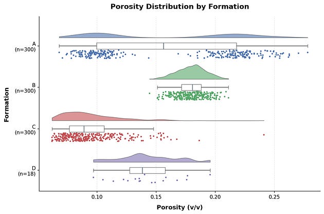
Another tidied up version of the raincloud plot that would be more suited for including in apublication.
The split matters more than the individual styling choices. Layer properties, like the box line weight and median colour, go through the prefixed kwargs.
Everything that belongs to the axes rather than a layer, such as labels, title, gridlines, and the tick text, is plain matplotlib after the raincloud plot call.
The sample counts under each formation name do the same work the rain does, but provides an instant number for the reader and saves them having to count each point (very few people will do that!).
This is also where you meet the limits of ptitprince’s raincloud plot. If you need to restyle an element the kwargs don’t reach and you then end up digging through the axes’ children to find it, and at that point the hand-built version from the previous article can appear to be less work, not more.
The Parameter That Changes the Interpretation of the Cloud
One argument is worth singling out when creating the raincloud plot, because it can change what the chart says rather than how it looks.
bw sets the bandwidth of the kernel density estimate behind the cloud, and it controls how much smoothing is applied to the shape you see.
fig, axs = plt.subplots(1, 3, figsize=(12, 4), sharey=True)
for ax, bw in zip(axs, [0.1, 0.3, 0.8]):
    pt.RainCloud(x="formation", y="porosity",
                 data=data[data.formation == "A"],
                 orient="h", ax=ax, bw=bw, move=0.2, point_size=2.5)
    ax.set_title(f"bw = {bw}")
    ax.set_xlabel("Porosity (frac)")
    ax.set_ylabel("")
axs[0].set_ylabel("Formation")
plt.tight_layout()
The same bimodal formation drawn at three bandwidths. Two sharp humps at 0.1, two clear humps at 0.3, one broad hump at 0.8
This is the same formation A in all three panels.
At a bandwidth of 0.1 the two populations are sharp and separate.
At 0.3 they are still clearly there.
At 0.8 they have merged into one broad hump, and the cloud now tells you this is a single, wide distribution.
For a petrophysicist that is the difference between one lithology and a mixed zone, decided by a single smoothing parameter.
The rain is the safeguard, because the two clusters of points stay where they are, no matter what the smoothing does. If the cloud and the rain disagree about how many populations you have, then we should believe the rain.
When To Use ptitprince or matplotlib
For exploratory work the ptitprince library is an easy choice. One call gets you a complete, readable raincloud for a first look at new data or a quick comparison across formations, and move plus a couple of styling arguments carry it a long way. With axes-level polish on top, it will take you all the way to a publication figure too.
The hand-built version is for when the wrapper gets in the way, for example when an element the prefixed kwargs can’t reach, or an environment where a thinly maintained dependency is more trouble than thirty lines of matplotlib you own and can control.
Either way, the same rule from the previous article applies, and figure 4 is the reason: the cloud is an estimate and the rain is the data. Whichever tool draws the chart, when the two disagree, believe the rain.
Throughout this article I have mentioned the hand-built version as the fallback for when the wrapper gets in the way. If you want to see how that works, I have written a full walkthrough on Substack where I build the raincloud plot from scratch in matplotlib, layer by layer, using the same four-formation dataset as this article.
→ From Boxplot to Raincloud: Building a Better Distribution Plot in Python