

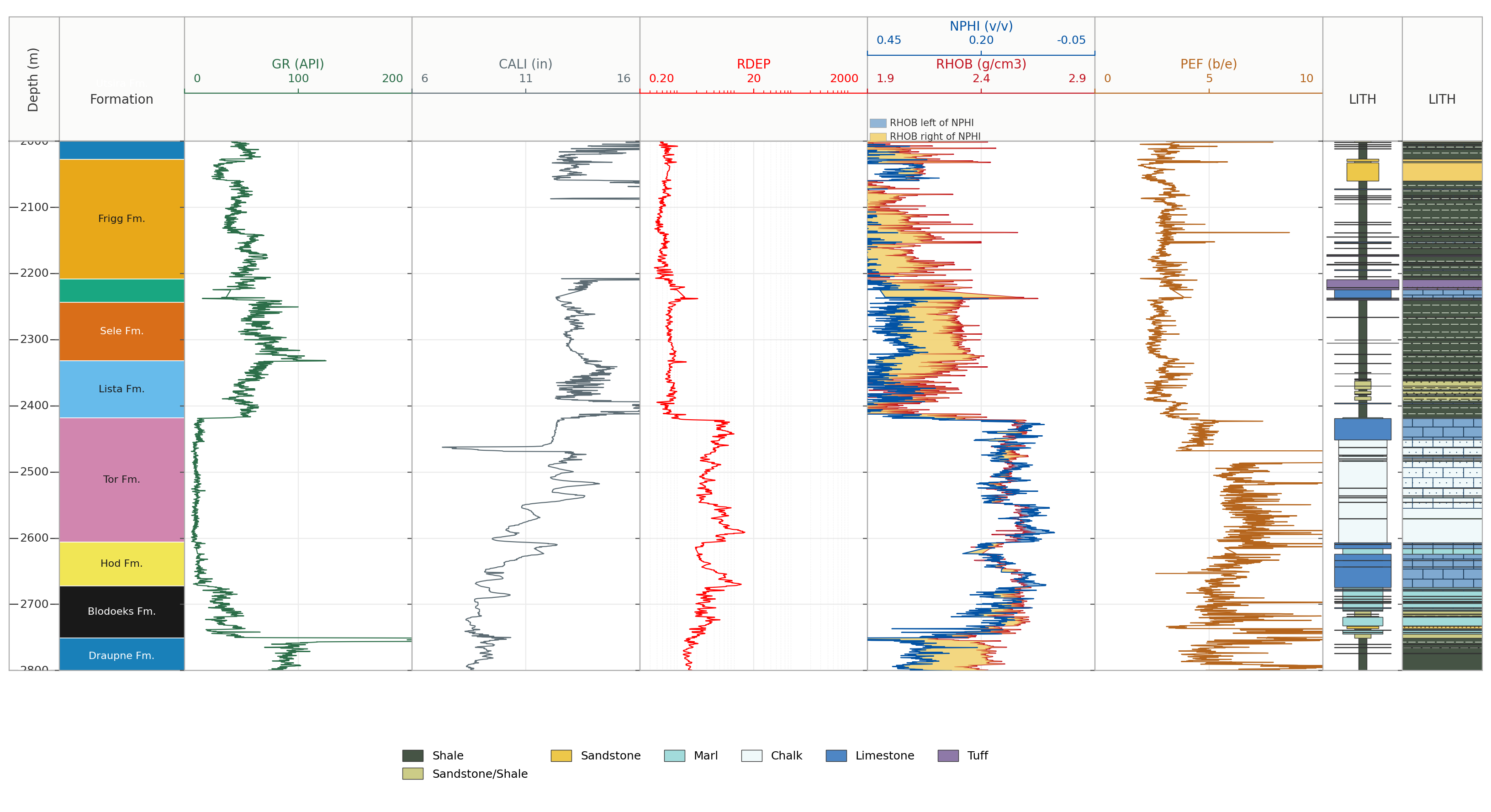
Back in 2020, I published my first article on working with well log data and displaying it using Matplotlib in Python. Since then, I have explored many different aspects of matplotlib and how it can be used for working with well logs, including displaying LWD Image Data and Lithology Data. I even spent time working out how to display shading between neutron and density logs, which are both on separate scales and units, and I remember it was quite a headache at the time!
These were explored and written before ChatGPT came onto the scene, so I often relied heavily on Stackoverflow back then. I wouldn’t be surprised if many of my early articles have made it into the training data for LLMs.
Matplotlib is one of my favourite Python plotting libraries. It may not be the prettiest plotting library out of the box, but with a few extra lines of code you can usually get a plot looking the way you want it. Mostly!
Over the years, I have made several attempts at building my own Python library for well log plotting. Most of these attempts never made it much beyond a collection of scripts, experiments and half-finished ideas.
Recently, I decided to revisit those old attempts and see whether Claude could help turn some of my existing code and unfinished ideas into something more complete.
The aim was to create a library that was easy to use, but still flexible enough to handle the things that regularly come up when plotting well logs, including different log types, curve fills and shading, lithology patterns and multi-track layouts.
That eventually became PetroPlots.
Full docs can be found here: https://petroplots.readthedocs.io/en/latest/
Even though Claude and other LLMs can easily build a plot, what I have found is there is often a lack of consistency in what it generates. So this library, may one day shortly be used by LLMs when building their plots. Not only that, this also completes something that I have been trying to sort out for the last few years.
Why Build Another Plotting Library?
There are already several Python libraries available for working with well log data, so the aim with PetroPlots was not to replace them.
Instead, I wanted to tackle one particular part of the workflow: creating well log plots without having to rewrite the same matplotlib code each time or getting Claude to generate it, which resulted in slight differences each time.
A typical well log plot can quickly become quite complicated. We may have several tracks, curves with different scales, reversed axes, logarithmic curves, fills between curves, lithology columns, formation tops and a shared depth axis.
None of these are difficult to create in matplotlib. The problem is that there are quite a few small pieces that need to be set up each time, which can be time consuming.
PetroPlots tries to handle that repetitive part while still returning a normal matplotlib figure that can be modified afterwards.
When designing the library I wanted it to allow you to easily build up a plot, track by track, and curve by curve without having to know detailed matplotlib calls. One other crucial area I wanted the library to tackle was the ability to use templates that were very simple to use, maintain and read.
If you want to try it out, read on.
Installing PetroPlots
PetroPlots can be installed using pip:
pip install petroplotsIt requires Python 3.10 or newer, with Matplotlib, NumPy and pandas forming the core dependencies. Additional packages such as lasio are optional and only needed for certain functionality.
Once installed, we can import the library:
import petroplots as ppFor the examples here, I will use the synthetic example dataset included with the library.
df = pp.datasets.load_example()The important point is that PetroPlots works primarily with pandas DataFrames. This means it can sit alongside whatever process you already use to load, clean or manipulate your well log data.
Creating a Basic Well Log Plot
Let’s start with a simple gamma ray track.
plot = pp.LogPlot(df, top=2000, bottom=2100)

gr = plot.add_track()
gr.add_curve("GR", limits=(0, 150), units="API")

fig, axes = plot.render() 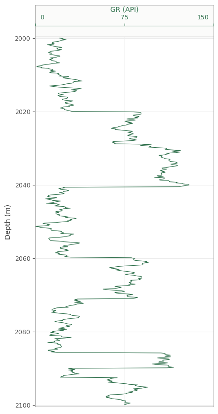
Instead of working directly with matplotlib axes, we first create a LogPlot, add tracks to it and then add curves to those tracks.
Calling render() then creates the matplotlib figure.
This separation turned out to be quite useful during development. Rather than immediately drawing everything onto a figure, PetroPlots first builds a description of what the plot should contain.
We can then add more tracks before rendering the final figure.
plot = pp.LogPlot(df, top=2000, bottom=2100)

plot.add_depth(interval=10)

gr = plot.add_track()
gr.add_curve("GR", limits=(0, 150), units="API")

res = plot.add_track()
res.add_curve("RT", limits=(0.2, 2000), units="ohm.m", scale="log")

fig, axes = plot.render()
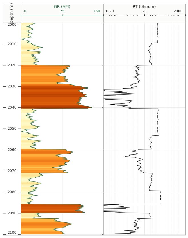
When we run the code, we get the following plot. Please note that the resistivity is synthetic, which accounts for the “odd” shape and style.
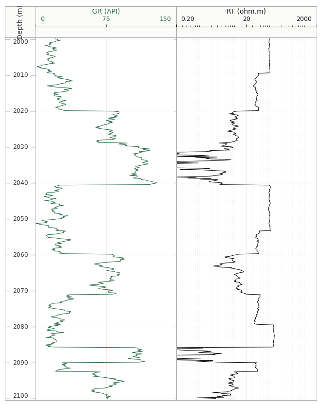
The depth axis is shared between the tracks and increases downwards, as we would normally expect for a well log display.
PetroPlots also contains conventions for common curve families, so limits, scale and direction can often be inferred automatically. For example, resistivity curves can be placed on a logarithmic scale and neutron porosity can run from higher values on the left to lower values on the right.
Putting Multiple Curves on a Track
Many petrophysical plots contain more than one curve within the same track.
A common example is density and neutron porosity.
plot = pp.LogPlot(df, top=2000, bottom=2100)

plot.add_depth(interval=10)

gr = plot.add_track()
gr.add_curve("GR", limits=(0, 150), units="API")

res = plot.add_track()
res.add_curve("RT", limits=(0.2, 2000), units="ohm.m", scale="log")

nd = plot.add_track()
nd.add_curve("RHOB", limits=(1.9, 2.9), units="g/cm3")
nd.add_curve("NPHI", limits=(0.45, -0.05), units="v/v")

fig, axes = plot.render()
Even though these curves have completely different units and scales, they can still be displayed together.
Bear in mind this is a completely synthetic dataset, so it may not make sense petrophysically, and is used to illustrate the process.
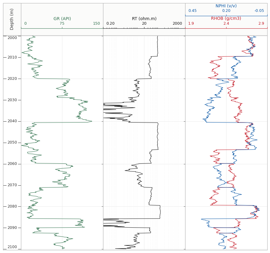
We can then add crossover shading after adding the curves to the nd track, but before the final plot.render()
nd.crossover()
This is one of those things that looks simple on a finished plot but requires a little more care behind the scenes due to the different units and scale ranges.
Density and neutron curves are recorded using different units and numerical ranges. PetroPlots therefore compares them in their normalised display space before determining where the crossover occurs.
That means the shading represents where the curves actually cross on the plot, rather than where their raw numerical values happen to cross.
Adding Fills and Shading
Filling between curves is another thing I use regularly when creating well log plots.
For example, we can shade between two porosity curves:
phi = plot.add_track()
phi.add_curve("PHIT", limits=(0.4, 0))
phi.add_curve("PHIE", limits=(0.4, 0))

phi.fill("PHIE", "PHIT")
A fill can also be made between a curve and a fixed value.
gr.fill(baseline=0, cmap="YlOrBr")
or:
sw.fill(left="SW", right=1.0)
This allows several common log presentation styles to be built without having to manually create the masks and fill_betweenx calls each time.
Adding Lithology
Lithology tracks were one of the main things I wanted PetroPlots to handle.
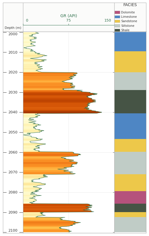
Colouring a categorical column is relatively straightforward. Where things become more interesting is when we want colours to remain consistent between wells.
Imagine one well contains sandstone, shale and limestone, while another contains only sandstone and shale. If the colour mapping is generated independently from the values present in each well, the same lithology can potentially end up with a different colour.
PetroPlots uses a FaciesScheme that defines the complete set of classes before the data are plotted. This keeps the relationship between a class and its colour fixed across plots.
For example:
plot.add_facies("FACIES", pp.LITHOLOGY)
PetroPlots also includes a second lithology scheme containing geological ornament:
plot.add_facies("FACIES", pp.LITHOLOGY_FGDC)
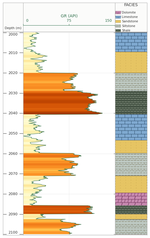
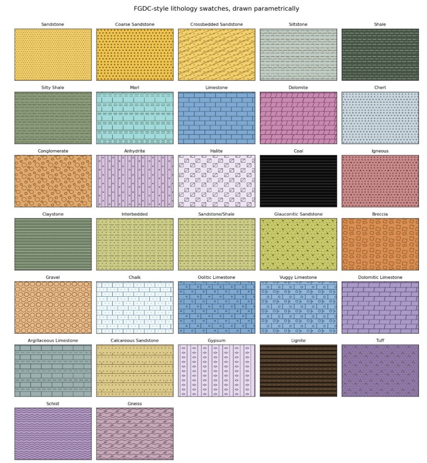
The library currently contains 30 parametric patterns and 32 named lithologies inspired by the FGDC geological map symbol standard. The patterns are generated as geometry rather than raster images, which means they remain vector graphics when plots are exported to formats such as PDF or SVG.
Custom schemes can also be created.
scheme = pp.FaciesScheme.from_lithologies(
    ["Shale", "Sandstone", "Limestone", "Dolomite"]
)
This was important as lithology naming is often different between projects.
Formation Tops
We can also add formation information to the data and use it within the log plot.
df = pp.add_tops(df, "field_tops.csv", well="15/9-19 A")
PetroPlots can read tops from several different structures and file formats, including DataFrames, mappings, CSV, Excel, JSON and Parquet. The resulting formation column is ordered according to depth rather than alphabetically.
Once formation information has been added, a zone track can be included:
plot.add_zones()
The formation names are then displayed alongside the log tracks.
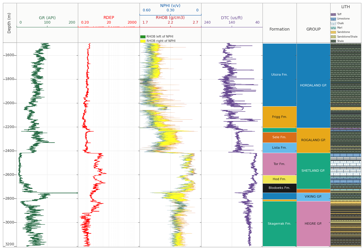
This also means the same formation information can be used elsewhere, such as splitting crossplots into panels.
More Than Well Log Plots
Although well log plots were the original motivation for the library, I also wanted some consistency when moving between different types of figures. You may have seen that I enjoy writing and exploring different types of plots and how to manipulate them to make them suitable for publishing or sharing.
PetroPlots therefore includes crossplots and histograms.
For example:
pp.crossplot(df, "NPHI", "RHOB", color="GR")
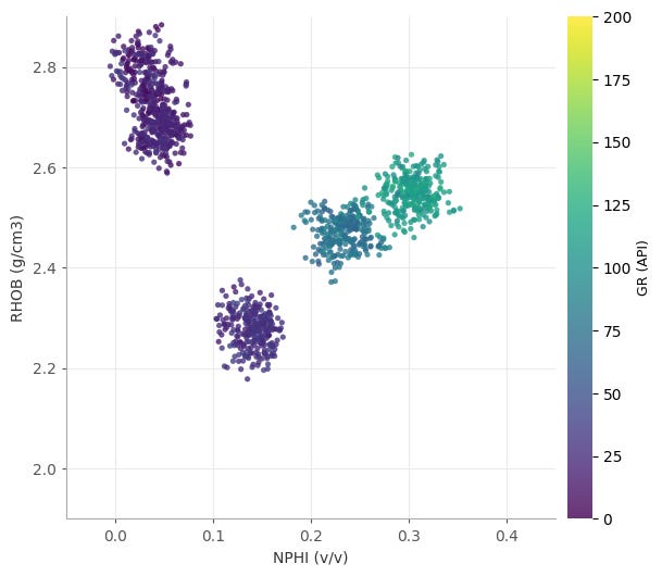
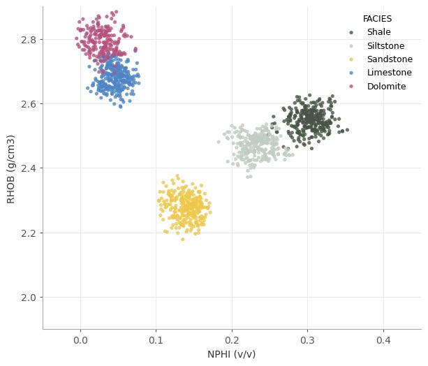
We could instead colour the points by facies:
pp.crossplot(
    df,
    "NPHI",
    "RHOB",
    color="FACIES",
    scheme=pp.LITHOLOGY
)
Or create a histogram using the same facies scheme:
pp.histogram(
    df,
    "RHOB",
    color="FACIES",
    scheme=pp.LITHOLOGY
)
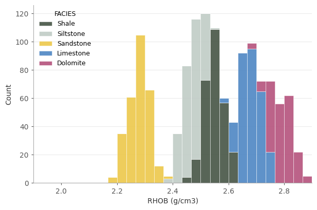
The idea here is maintaining consistency. If sandstone is represented by a particular colour in a log plot, it should remain that colour when we move to a crossplot or histogram. Curve conventions are also carried across plot types, including logarithmic treatment of variables such as permeability.
Splitting Data Into Multiple Panels
Another feature I have found useful is creating small multiples.
For example, a crossplot can be split by formation:
pp.crossplot(
    df,
    "NPHI",
    "RHOB",
    by="FACIES",
    color="GR"
)
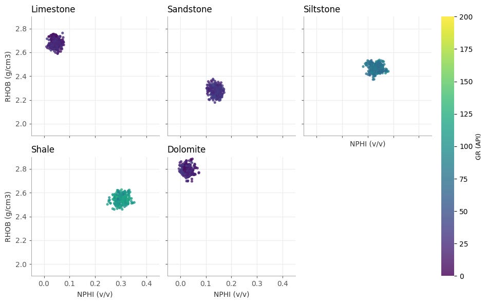
Rather than allowing every subplot to calculate its own limits, PetroPlots calculates the common plotting ranges before splitting the data.
This is a small detail, but an important one.
If every panel autoscaled independently, two very different distributions could end up looking surprisingly similar. Keeping the same axes across panels makes the comparison between groups much more meaningful.
Creating Reusable Templates
One problem with well log plotting is that we often want to generate the same layout for many wells.
That led to templates, which are maintained through simple YAML files.
For example:
version: 1
name: triple_combo
depth: DEPTH
tracks:
  - type: curve
    curves: [GR]
    limits: [0, 200]
    units: {GR: API}
  - type: fill
    curves: [RHOB, NPHI]
    limits:
      RHOB: [1.9, 2.9]
      NPHI: [0.45, -0.05]
    crossover: true
  - type: facies
    curve: FACIES
    scheme: lithology_fgdc
    style: patches
    width: 0.4
A template defines the curves and tracks that should appear rather than being tied to a particular DataFrame.
PetroPlots also includes curve aliases. This means a template asking for GR can resolve a dataset containing an alternative recognised name such as SGR.
More importantly, a missing curve does not necessarily cause the complete plot to fail.
If a track cannot be created because its curve is missing, the track can be dropped. If one side of a density-neutron crossover is unavailable, it can fall back to displaying the remaining curve.
That makes templates much more useful when running across collections of wells where curve availability is rarely identical.
Plots can also be saved as templates:
pp.save_template(plot, "my_template.yaml")
It Is Still Matplotlib
One thing I didn’t want PetroPlots to do was hide Matplotlib completely.
After rendering a figure, PetroPlots returns the Matplotlib figure and its axes.
fig, axes = plot.render()We can then carry on modifying the plot using normal Matplotlib commands.
For example:
axes["GR"].axvline(75, ls="--", color="0.4")
axes[0].set_facecolor("#FAFAFA")
PetroPlots is therefore more of a layer on top of Matplotlib rather than a replacement for it.
That was an important design decision for me.
There will always be something slightly unusual that needs changing on a figure, and trying to expose every possible Matplotlib option through another API would probably create a library more complicated than Matplotlib itself.
At that point we would have rather spectacularly missed the point.
Loading LAS Data
PetroPlots is primarily a plotting library rather than a well data management library.
However, there is a small convenience wrapper around lasio:
df = pp.io.from_las("example.las")This requires the optional LAS dependency:
pip install "petroplots[las]"For DataFrames that have already been loaded elsewhere, normalise() can clean up some of the common differences in how log data are structured:
df = pp.io.normalise(df, depth="DEPT")This can move depth from the index into a column, replace common null values such as -999.25 with NaN, and check that depth is monotonic.
There is deliberately no attempt to turn PetroPlots into another complete well data framework. Libraries such as lasio, welly and dlisio already deal with those areas.
Building It With Claude
One of the interesting parts of this project for me has been how it was developed.
PetroPlots did not start from a blank prompt asking Claude to build a Python library.
I already had years of plotting examples, experiments and partially completed attempts at creating something similar. What Claude helped with was taking those ideas and turning them into a much more coherent result.
There was still plenty of back and forth.
Some features sounded sensible until I actually plotted real examples. Others worked technically but produced figures that I did not like. There were also decisions around API design, default behaviour, testing and what functionality should deliberately be left out.
That is probably the part of AI-assisted development I find most interesting.
The value was not that I no longer had to understand the problem. If anything, I needed to be clearer about what I wanted the library to do.
What changed was how quickly I could explore an idea, test it, decide it was terrible, throw it away and try another approach.
For a project containing several years’ worth of unfinished code, that made quite a difference.
Where Next?
PetroPlots is still a young project and there are plenty of areas I want to explore further.
Check it out on Github
https://github.com/andymcdgeo/petroplots
And the docs can be found here:
https://petroplots.readthedocs.io/en/latest/
For now, though, it does the main thing I originally wanted it to do: take away much of the repetitive setup involved in making well log plots while still leaving Matplotlib available underneath.
The library currently supports multi-track well log plots, curve fills and crossovers, facies and lithology tracks, formation zones, crossplots, histograms, small multiples and reusable plot templates.
More importantly, I can finally stop creating another folder called something like:
well_plotting_library_final_v3_really_final
before abandoning it six weeks later.
If you do try it out, please feel free to drop a comment here. Or if you encounter any issues, feel free to raise them as an issue over on Github.
In the meantime, happy plotting.