


Understanding data completeness, is an essential part of any data analysis workflow. In the case of well log data, we often have similarly acquired datasets in multiple wells. One way I like to check this is by using a completeness heatmap.
At a glance the data completeness heatmap tells you which curves (or columns) you have across multiple measurement locations. In this example we are using different wells.
Form this we can also tell which curves are missing from which wells, and whether the gaps are concentrated in a particular formation or scattered across the well.
In my previous article, I have focused on how to improve the look of static matplotlib figures and there is a problem with them.
That problem is that static figures, even well-made ones, make your brain work to answer follow-up questions. In cases where we have a large amount of columns and rows in our heatmap, you simply can’t hover over a cell and see exactly which well (row) and curve (column) combination you’re looking at. Instead you have to look up which column and row you are in.
Plotly, another excellent Python plotting library fixes most of that.
In this article we will walk through building an interactive well log completeness heatmap from scratch, with hover tooltips, cell labels, white borders, and a multi-formation panel.
Although this example uses well log data, the same approach works anywhere you need to compare data completeness across repeated measurement locations, whether that means wells, stations, assets, samples, or sites.
The Data
First, we will create a dataset. This dataset is a synthetic set of 8 wells, 10 curves, and 4 formations. Ideally, you would need to load and compute these completeness values fo your own dataset.
import pandas as pd

wells  = [’Ardmore-1’, ‘Ardmore-4’, ‘Brindal-1’, ‘Brindal-3’,
          ‘Brindal-5’, ‘Brindal-8’, ‘Caxton-2’,  ‘Caxton-6’]

curves = [’GR’, ‘RDEP’, ‘RSHA’, ‘RHOB’, ‘NPHI’, ‘DTC’, ‘DTS’, ‘PEF’, ‘CALI’, ‘SP’]

completeness_data = {
    ‘Thornfield’: [
        [100.0, 100.0, 100.0, 26.2, 100.0, 40.8, 61.5, 49.5, 100.0, 54.0],  # Ardmore-1
        [100.0, 100.0, 100.0, 28.0, 100.0, 37.2, 60.8, 52.8, 100.0, 54.5],  # Ardmore-4
        [100.0, 100.0, 100.0, 31.5, 100.0, 38.8, 59.8, 50.5, 100.0, 54.0],  # Brindal-1
        [100.0, 100.0, 100.0, 29.8, 100.0, 41.5, 60.0, 46.5, 100.0, 52.8],  # Brindal-3
        [100.0, 100.0, 100.0, 30.2, 100.0, 37.5, 59.0, 52.2, 100.0, 56.5],  # Brindal-5
        [100.0, 100.0, 100.0, 31.0, 100.0, 40.2, 59.0, 53.5, 100.0, 55.8],  # Brindal-8
        [100.0, 100.0, 100.0, 35.2, 100.0, 37.5, 58.0, 50.7, 100.0, 54.8],  # Caxton-2
        [100.0, 100.0, 100.0, 31.0, 100.0, 43.2, 62.5, 46.5, 100.0, 54.2],  # Caxton-6
    ],
    ‘Veldwick’: [
        [100.0, 100.0, 100.0, 75.0, 100.0, 65.1, 59.8, 52.1, 100.0, 57.9],  # Ardmore-1
        [100.0, 100.0, 100.0, 87.0, 100.0, 73.8, 60.1, 47.8, 100.0, 53.2],  # Ardmore-4
        [100.0, 100.0, 100.0, 84.0, 100.0, 72.0, 62.0, 50.2, 100.0, 58.1],  # Brindal-1
        [100.0, 100.0, 100.0, 82.0, 100.0, 69.6, 62.6, 49.9, 100.0, 56.4],  # Brindal-3
        [100.0, 100.0, 100.0, 81.5, 100.0, 69.9, 59.6, 50.1, 100.0, 52.8],  # Brindal-5
        [100.0, 100.0, 100.0, 88.6, 100.0, 73.5, 59.4, 49.0, 100.0, 55.6],  # Brindal-8
        [100.0, 100.0, 100.0, 75.1, 100.0, 64.5, 59.6, 49.4, 100.0, 58.2],  # Caxton-2
        [100.0, 100.0, 100.0, 84.9, 100.0, 73.0, 61.0, 47.5, 100.0, 55.4],  # Caxton-6
    ],
    ‘Oskarby’: [
        [100.0, 100.0, 100.0, 100.0, 100.0, 100.0, 80.4, 84.4, 100.0, 52.8],  # Ardmore-1
        [100.0, 100.0, 100.0, 100.0, 100.0, 100.0, 85.5, 93.4, 100.0, 58.3],  # Ardmore-4
        [100.0, 100.0, 100.0, 100.0, 100.0, 100.0, 84.1, 91.2, 100.0, 52.3],  # Brindal-1
        [100.0, 100.0, 100.0, 100.0, 100.0, 100.0, 83.2, 90.9, 100.0, 56.1],  # Brindal-3
        [100.0, 100.0, 100.0, 100.0, 100.0, 100.0, 84.0, 88.9, 100.0, 54.3],  # Brindal-5
        [100.0, 100.0, 100.0, 100.0, 100.0, 100.0, 88.6, 93.4, 100.0, 53.7],  # Brindal-8
        [100.0, 100.0, 100.0, 100.0, 100.0, 100.0, 80.3, 86.3, 100.0, 53.3],  # Caxton-2
        [100.0, 100.0, 100.0, 100.0, 100.0, 100.0, 86.2, 91.3, 100.0, 55.0],  # Caxton-6
    ],
    ‘Dravenport’: [
        [100.0, 100.0, 100.0,  80.0,  80.0, 100.0, 100.0, 100.0, 100.0, 54.5],  # Ardmore-1
        [100.0, 100.0, 100.0, 100.0, 100.0, 100.0, 100.0, 100.0, 100.0, 56.5],  # Ardmore-4
        [100.0, 100.0, 100.0, 100.0, 100.0, 100.0, 100.0, 100.0, 100.0, 52.8],  # Brindal-1
        [100.0, 100.0, 100.0,  80.0,  80.0, 100.0, 100.0, 100.0, 100.0, 55.8],  # Brindal-3
        [100.0, 100.0, 100.0, 100.0, 100.0, 100.0, 100.0, 100.0, 100.0, 52.5],  # Brindal-5
        [100.0, 100.0, 100.0, 100.0, 100.0, 100.0, 100.0, 100.0, 100.0, 52.8],  # Brindal-8
        [100.0, 100.0, 100.0,  80.0,  80.0, 100.0, 100.0, 100.0, 100.0, 55.2],  # Caxton-2
        [100.0, 100.0, 100.0, 100.0, 100.0, 100.0, 100.0, 100.0, 100.0, 55.9],  # Caxton-6
    ],
}
One line to turn that into the results dict the rest of the article uses. In this dictionary we have a pandas dataframe per formation, wells as rows, curves as columns:
results = {
    formation: pd.DataFrame(matrix, index=wells, columns=curves)
    for formation, matrix in completeness_data.items()
}

formation_names = list(results.keys())
Displaying the Basic Heatmap with px.imshow()
To begin displaying our heatmap we can call upon px.imshow() .
px.imshow() is Plotly Express’s equivalent of matplotlib’s ax.imshow(). You pass it a 2D array or dataframe and it renders a colour-mapped grid.
import plotly.express as px

completeness_pivot = results[’Veldwick’]
fig = px.imshow(
    completeness_pivot,
    color_continuous_scale=”RdYlGn”,
    zmin=0,
    zmax=100,
    labels={”color”: “Completeness (%)”},
    title=”Well Log Completeness - Veldwick”,
)
fig.show()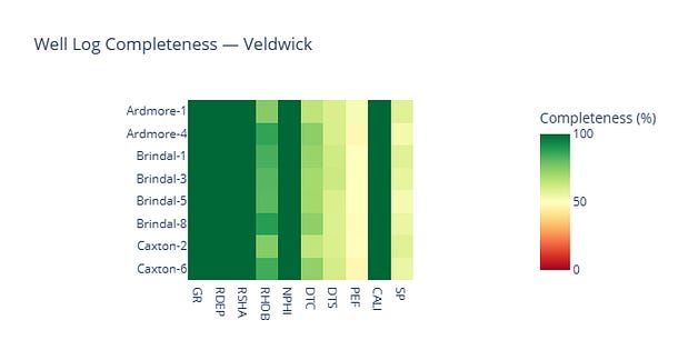
Single-formation completeness heatmap for Veldwick using px.imshow().
The zmin and zmax arguments pin the colour scale to 0-100, which matters when you’re comparing formations.
Without these values being defined, Plotly autoscales to the data range.
Adding Hover Tooltips
By default px.imshow() shows the x, y, and z values on hover.
To control exactly what appears, and how it’s formatted we need to pass a hovertemplate via update_traces. The formatting can include regular HTML syntax, which makes it easy to style, and we can easily call upon the x and y values with %{y} , which is the well (row) and %{x} which is the curve (column).
fig = px.imshow(
    completeness_pivot,
    color_continuous_scale=”RdYlGn”,
    zmin=0,
    zmax=100,
    labels={”color”: “Completeness (%)”},
    title=”Well Log Completeness — Veldwick”,
)

fig.update_traces(
    hovertemplate=(
        “<b>Well:</b> %{y}<br>”
        “<b>Curve:</b> %{x}<br>”
        “<b>Completeness:</b> %{z:.1f}%<extra></extra>”
    ),
)
fig.show()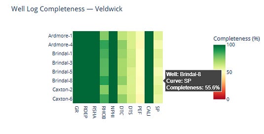
The <extra></extra> tag removes the trace name Plotly appends by default.
%{z:.1f} formats the data values to one decimal place, which is enough precision to be useful for this figure.
Cell Labels and Borders
The hover tooltip is useful when you’re exploring, but for a published figure it helps to have the percentages visible directly on the chart, in the same way the matplotlib version had annotations in each cell.
We can do this using texttemplate.
Also, by adding xgap and ygap we can add pixel-width gaps between cells, which Plotly fills with the background colour. Set the background to white and you get clean white borders.
fig = px.imshow(
    completeness_pivot,
    color_continuous_scale=”RdYlGn”,
    zmin=0,
    zmax=100,
    labels={”color”: “Completeness (%)”},
    title=”Well Log Completeness — Veldwick”,
)

fig.update_traces(
    xgap=2,
    ygap=2,
    texttemplate=”%{z:.0f}%”,
    textfont={”size”: 10},
    hovertemplate=(
        “<b>Well:</b> %{y}<br>”
        “<b>Curve:</b> %{x}<br>”
        “<b>Completeness:</b> %{z:.1f}%<extra></extra>”
    ),
)
fig.update_layout(
    xaxis_title=”Curve”,
    yaxis_title=”Well”,
    font={”family”: “monospace”},
    plot_bgcolor=”white”,
    paper_bgcolor=”white”,
    width=900,
    height=500,
)
fig.show()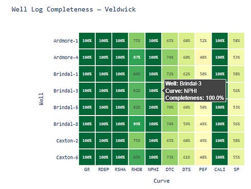
%{z:.0f}% in the cell label rounds to a whole number, which can avoid unnecessary decimal places. The monospace font stops the percentage values shifting around as the digit count changes across cells.
Switching Formations with a Dropdown
In a Jupyter notebook, you can wire the figure up to a formation selector using ipywidgets.
The @interact decorator creates a dropdown from the list and re-runs the function every time the selection changes. The figure title updates automatically since the formation name is passed as a variable.
I find this a great way to switch between different formations or groups of data, especially when we are dealing with a large number of groups.
from ipywidgets import interact

@interact(formation=formation_names)
def plot_formation(formation=’Veldwick’):
    pivot = results[formation]
    fig = px.imshow(
        pivot,
        color_continuous_scale=”RdYlGn”,
        zmin=0,
        zmax=100,
        labels={”color”: “Completeness (%)”},
        title=f”Well Log Completeness - {formation}”,
    )
    fig.update_traces(
        xgap=2,
        ygap=2,
        texttemplate=”%{z:.0f}%”,
        textfont={”size”: 10},
        hovertemplate=(
            “<b>Well:</b> %{y}<br>”
            “<b>Curve:</b> %{x}<br>”
            “<b>Completeness:</b> %{z:.1f}%<extra></extra>”
        ),
    )
    fig.update_layout(
        xaxis_title=”Curve”,
        yaxis_title=”Well”,
        font={”family”: “monospace”},
        plot_bgcolor=”white”,
        paper_bgcolor=”white”,
        width=900,
        height=500,
    )
    fig.show()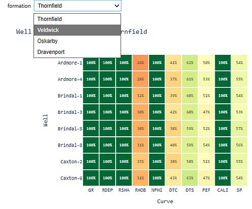
This is a Jupyter-specific feature and it won’t work in a plain Python script or Streamlit app.
For Streamlit, the equivalent is st.selectbox, which feeds into a similar function. The multi-formation panel in the next section is a better fit if you want all four formations visible at once.
Faceting Across Formations
The matplotlib version handled multiple formations with a subplot grid, where we have one axis per formation, arranged in a column.
Although px.imshow() supports some faceting use cases, in this example I am going to use plotly.graph_objects with make_subplots, because we already have one 2D table per formation.
The results dict from the data section already has one pivot per formation, so no reshaping needed.
We can build the subplot figure using make_subplots, and then adding a Heatmap trace for each formation:
from plotly.subplots import make_subplots
import plotly.graph_objects as go

fig = make_subplots(
    rows=len(formation_names),
    cols=1,
    subplot_titles=list(formation_names),
    shared_xaxes=True,
    vertical_spacing=0.06,
)
for i, formation in enumerate(formation_names, start=1):
    pivot = results[formation]
    z_vals = pivot.values
    fig.add_trace(
        go.Heatmap(
            z=z_vals,
            x=pivot.columns.tolist(),
            y=pivot.index.tolist(),
            colorscale=”RdYlGn”,
            zmin=0,
            zmax=100,
            xgap=2,
            ygap=2,
            showscale=(i == 1),
            colorbar=dict(
                title=”Completeness (%)”,
                len=0.25,
                y=0.88,
            ) if i == 1 else {},
            text=[[f”{v:.0f}%” for v in row] for row in z_vals],
            texttemplate=”%{text}”,
            textfont={”size”: 9, “family”: “monospace”},
            hovertemplate=(
                “<b>Well:</b> %{y}<br>”
                “<b>Curve:</b> %{x}<br>”
                “<b>Formation:</b> “ + formation + “<br>”
                “<b>Completeness:</b> %{z:.1f}%<extra></extra>”
            ),
        ),
        row=i,
        col=1,
    )
fig.update_layout(
    height=290 * len(formation_names),
    title_text=”Well Log Completeness by Formation”,
    title_font_size=16,
    font={”family”: “monospace”},
    plot_bgcolor=”white”,
    paper_bgcolor=”white”,
)
fig.show()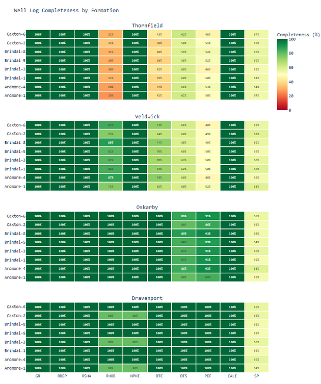
Four-panel stacked heatmap (Thornfield, Veldwick, Oskarby, Dravenport) with white cell borders, percentage labels, shared x-axis, and formation-aware hover tooltips
The shared_xaxes=True argument keeps curve columns aligned across formations so that the same curve appears in the same column regardless of which panel you’re looking at, which makes vertical comparison straightforward.
The showscale logic avoids repeating the colour bar across every subplot.
Embedding in Streamlit
If you’re building a well review tool or a data QC dashboard, the Plotly figure drops into Streamlit with a single call:
import streamlit as st

st.title(”Well Log Completeness Review”)
st.plotly_chart(fig, use_container_width=True)
use_container_width=True makes the figure fill the column width, which looks better than Plotly’s fixed default.
From there you can wire up Streamlit widgets such as formation selectors, well filters, a date picker and the figure will rebuild.
This isn’t a Streamlit tutorial, so I’ll leave the wiring there. If you’re already working in Streamlit, the move from notebook figure to deployed tool is not much work.
What the Switch to Plotly Actually Changes
In a static heatmap, checking a specific cell means tracing the row and column yourself. That works for small plots, but it becomes slower as the number of wells, curves, or groups increases. With Plotly, the hover tooltip brings the well, curve, formation, and completeness value directly to you.
There is still a trade-off. Static matplotlib figures are often better for reports, papers, and slide decks. Plotly is better when the figure is part of an active review, notebook workflow, or dashboard.