


PtitPrince can create a raincloud plot in a few lines of code. That is one of its main attractions, especially when you want a quick view of how several distributions compare.
The default output is useful for exploration, but it still looks like something produced inside a notebook. The layout can feel cramped, the labels come directly from the DataFrame, and the relative weight of the cloud, box and individual points is left to the library defaults. This may be fine whilst you are analysing the data, but less so when the figure needs to appear in a report, presentation or article.
To continue with my series on From Default to Publication Ready, this article will take the default PtitPrince output and improve it one step at a time. We will change the orientation, apply a more accessible colour palette, rebalance the components, improve the labels, remove unnecessary clutter and add sample sizes.
The idea is not to produce one perfect design, but to show the small decisions that can turn a basic working plot into a figure that can easily be included in a publication and communicates its message clearly.
If you are new to raincloud plots, I covered the individual components in an earlier article.
The data
For this article, we will generate some synthetic data that represents porosity distributions from four different geological formations.
The names and values are illustrative rather than real geology: two roughly normal distributions at different levels, one bimodal formation, and one that is skewed. This mix allows us to visualise different data distributions and to show the benefits of a raincloud plot
import numpy as np
import pandas as pd
import matplotlib.pyplot as plt
import ptitprince as pt

rng = np.random.default_rng(42)
formations = {
    "Vardan": rng.normal(0.21, 0.025, 400),
    "Kelvik": rng.normal(0.15, 0.02, 320),
    "Stenby": np.concatenate([rng.normal(0.10, 0.015, 20),
                              rng.normal(0.18, 0.015, 20)]),
    "Morvik": rng.beta(2, 5, 20) * 0.25,
}
df = pd.DataFrame(
    [(name, val) for name, vals in formations.items() for val in vals],
    columns=["Formation", "Porosity"],
)
With the data in place, we can call upon the raincloud plot like so:
f, ax = plt.subplots(figsize=(8, 6))
pt.RainCloud(x="Formation", y="Porosity", data=df, ax=ax)
plt.show()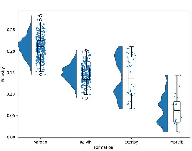
The default output is readable, however, the vertical layout squashes each cloud into a narrow column and we may start competing for space on the x-axis when we add more formations or formations with longer names.
Step 1: Flip the orientation
Raincloud plots often read better horizontally, in my opinion, particularly when the group labels are long or several distributions are being compared.
The cloud gets room to spread out and the rain falls in a wide band instead of a narrow vertical strip, and we can display the group names on the y axis, which can be great when we have long names and need to avoid rotating the labels.
f, ax = plt.subplots(figsize=(10, 7))
pt.RainCloud(x="Formation", y="Porosity", data=df, ax=ax,
             orient="h")
plt.show()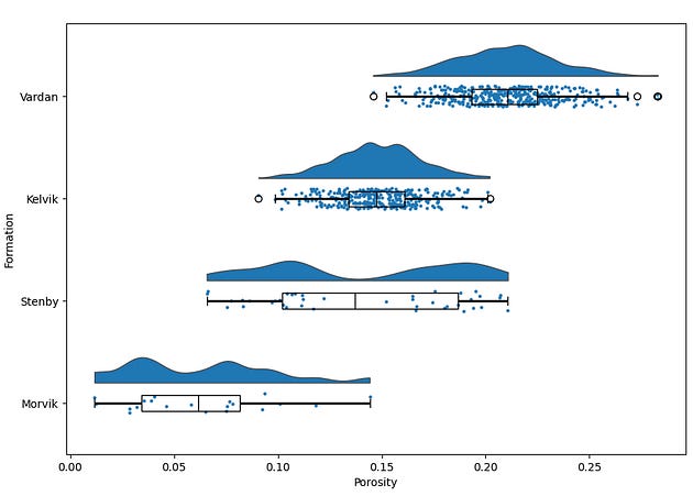
Horizontal raincloud plot giving each formation’s cloud and rain room to spread, with formation names on the y axis
We have also changed the figure size to give more width than height.
Step 2: Apply a colour palette
The default blue colour is fine if you want to keep the groups consistent, but sometimes it is good to be able to split the groups apart by colour, especially if we have a handful of groups.
We can easily apply a different colour palette, and it often helps to pick one that is easily accessible to readers, especially those that have varying forms of colour blindness. Additionally, adding a slight bit of transparency can also help soften the colours if they appear to harsh.
f, ax = plt.subplots(figsize=(10, 7))
pt.RainCloud(x="Formation", y="Porosity", data=df, ax=ax,
             orient="h",
             palette="colorblind", alpha=0.65)
plt.show()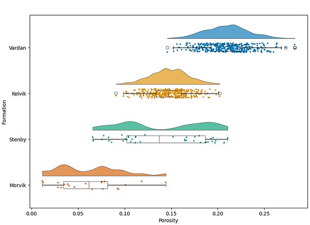
The same chart using seaborn’s colorblind palette with softened fill transparency
The colorblind palette ships with seaborn, so there’s nothing extra to install.
Step 3: Tune the cloud, the rain and the box
A raincloud plot consists of three components sharing a single axis, and the defaults for the plot give each component an arbitrary share of the space.
With a few width and jitter changes, we can rebalance them so the cloud dominates, the box stays a compact summary, and the rain forms a clear band underneath.
f, ax = plt.subplots(figsize=(10, 7))
pt.RainCloud(x="Formation", y="Porosity", data=df, ax=ax,
             orient="h",
             palette="colorblind", alpha=0.65,
             width_viol=0.7, width_box=0.25,
             point_size=3, jitter=0.08, move=0.25,
             box_showfliers=False)
plt.show()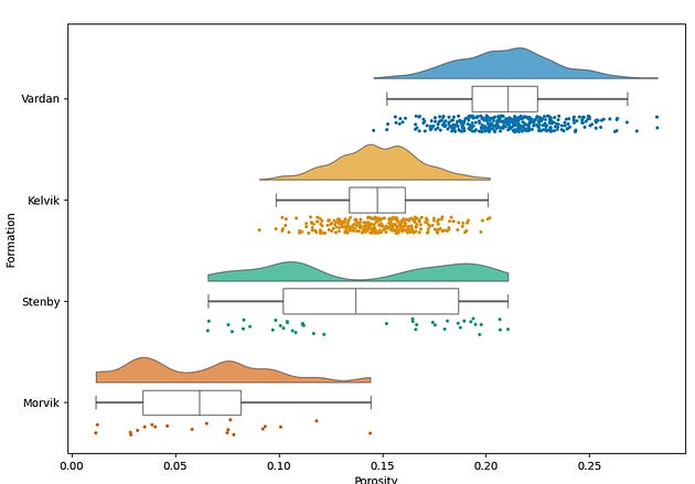
Rebalanced widths with a fuller cloud, slimmer box, smaller rain points, tighter jitter and no duplicate outlier markers
The values here are a reasonable starting point rather than a rule. width_viol and width_box control how much room the cloud and box take, point_size and jitter control how the rain reads, and move shifts the rain away from the box so the two don’t overprint. With more groups or more points per group, these tend to need another review.
The boxplot layer displays outlier markers by default. Setting box_showfliers=False removes them. In a raincloud plot, displaying them can amount to double counting because every observation, including the outliers, is already shown in the rain.
By having this on, matplotlib draws hollow circles for its outliers, exactly as a standalone boxplot would. In a raincloud that’s double counting: every point, outliers included, is already in the rain. The box’s outlier markers sit at the box position rather than in the rain band, so they read as extra data that isn’t there. ptitprince routes any argument prefixed with box_ through to the underlying boxplot, which is also how you’d pass other boxplot settings if you need them.
Rainclouds are one of a handful of chart types that most people never reach for, even when they’d tell the story far better than a histogram. I’ve covered three of them, with before and after examples on well log data, over on Substack. Link at the end.
Step 4: Say what the chart shows
The chart still labels its axes with DataFrame column names, which is not the best, especially if the names are more generic or contain special characters such as an underscore or dash.
We can tidy this up with a few small changes:
ax.set_xlabel("Porosity (v/v)", fontsize=12)
ax.set_ylabel("")
ax.set_title("Porosity Distribution by Formation",
             fontsize=14, fontweight="bold", loc="left", pad=15)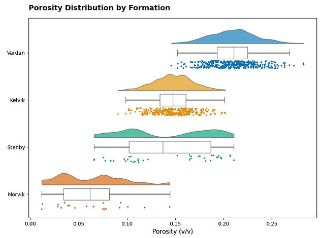
The empty y label is intentional. The formation names already tell the reader what that axis is, and a “Formation” label would repeat them.
For reports and presentations, a left-aligned title is easy to scan and works well on a wide figure. Journal figures often leave the title to the caption, so this is a design choice rather than a fixed rule.
Step 5: Remove what isn’t data
Matplotlib draws a full box around every plot by default. This is often considered “chart junk” by many and can make plots look ugly or distract the reader.
By adding light grid along the porosity axis we can help the reader’s eye across the chart. This is the quiet step that does the most for how finished the figure feels.
ax.spines[["top", "right"]].set_visible(False)
ax.xaxis.grid(True, linestyle="--", alpha=0.4)
ax.set_axisbelow(True)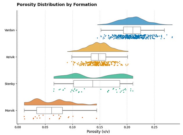
Labels and decluttering combined. Titled chart with axis units, open top and right spines, and a light dashed grid behind the data
set_axisbelow(True) pushes the gridlines behind the clouds and rain. Without it, dashed lines cut across your data, which can look messy.
Step 6: Show your sample sizes, then export properly
A raincloud plot invites the reader to trust the cloud, and the cloud is a smoothed estimate. When looking at the rain, it can also be difficult for the reader to estimate how many points are present for each group. For example between Vardan and Kelvik there are only 80 points difference, however, it would be difficult to know that by looking at the rain.
As a result the sample count is often worth putting directly on the figure, particularly when the groups are uneven. We can append the counts directly onto the group label on the y-axis rather than adding additional annotations.
counts = df.groupby("Formation", sort=False).size()
labels = [f"{name}\n(n={counts[name]})" for name in counts.index]
ax.set_yticks(ax.get_yticks())
ax.set_yticklabels(labels)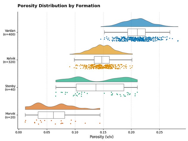
The finished figure. Publication-ready horizontal raincloud with sample counts under each formation name.
The Final Script
Here’s everything in one place, from data to exported figure.
import numpy as np
import pandas as pd
import matplotlib.pyplot as plt
import ptitprince as pt

rng = np.random.default_rng(42)
formations = {
    "Vardan": rng.normal(0.21, 0.025, 400),
    "Kelvik": rng.normal(0.15, 0.02, 320),
    "Stenby": np.concatenate([rng.normal(0.10, 0.015, 20),
                              rng.normal(0.18, 0.015, 20)]),
    "Morvik": rng.beta(2, 5, 20) * 0.25,
}
df = pd.DataFrame(
    [(name, val) for name, vals in formations.items() for val in vals],
    columns=["Formation", "Porosity"],
)
f, ax = plt.subplots(figsize=(10, 7))
pt.RainCloud(x="Formation", y="Porosity", data=df, ax=ax,
             orient="h",
             palette="colorblind", alpha=0.65,
             width_viol=0.7, width_box=0.25,
             point_size=3, jitter=0.08, move=0.25,
             box_showfliers=False)
ax.set_xlabel("Porosity (v/v)", fontsize=12)
ax.set_ylabel(")
ax.set_title("Porosity Distribution by Formation",
             fontsize=14, fontweight="bold", loc="left", pad=15)
ax.spines[["top", "right"]].set_visible(False)
ax.xaxis.grid(True, linestyle="--", alpha=0.4)
ax.set_axisbelow(True)
counts = df.groupby("Formation", sort=False).size()
labels = [f"{name}\n(n={counts[name]})" for name in counts.index]
ax.set_yticks(ax.get_yticks())
ax.set_yticklabels(labels)
plt.tight_layout()
plt.savefig("porosity_raincloud.png", dpi=600, bbox_inches="tight")
Closing Thoughts
The difference between a default raincloud plot and a finished figure is not a complicated block of code, but rather a series of small and deliberate choices.
Changing the orientation gives the distributions more room. Adjusting the palette and transparency can help improve readability. Tuning the cloud, box and rain makes each component contribute without competing for attention and for space. Clear labels provide context, while removing unnecessary spines and adding a light grid help the data stand out. Showing the sample sizes gives the reader a better sense of how much evidence sits behind each distribution.
Not every figure needs exactly the same settings. More groups, longer labels or larger datasets may require different dimensions, point sizes or spacing. The useful habit is to treat the default output as a starting point rather than the finished result.
One setting we have deliberately left untouched is the bandwidth used to estimate the cloud. That choice affects how smooth, noisy or even multimodal a distribution appears, and it can change the story the plot seems to tell. This was covered briefly in Raincloud Plots with PtitPrince: See What Your Data Is Really Doing.
Polishing a raincloud plot only pays off if the raincloud was the right chart to begin with. Alongside it sit ridgeline plots, bump charts and beeswarm plots. Over on Substack I’ve put together a piece covering all three, with before and after examples using well log data, so you can decide which one your data deserves.