


The boxplot is the common tool for comparing measurements across different geological formations, and it can also hide the thing you need to see. Boxplots reduce a distribution to five key numbers, so two formations with completely different shapes can produce similar looking boxes.
This is where raincloud plots can help. A raincloud plot stacks three views of a distribution in one: a half-violin for the shape (the “cloud”), the raw points jittered underneath (the “rain”), and a boxplot for the summary. You get the quick read of a boxplot without letting it hide what the data is actually doing.
Even though there there is a ready-made library for this in Python (ptitprince), we will be building one by hand using matplotlib. Once you have built it you can see precisely what the chart is showing.
The data
For this article, we will generate some synthetic data that represents porosity distributions from four different geological formations.
These distributions were chosen to show off the chart and may not necessarily represent real geology.
We can also import the required libraries, which are numpy, pandas, matplotlib and scipy.stats.
import numpy as np
import pandas as pd
import matplotlib.pyplot as plt
from scipy.stats import gaussian_kde

rng = np.random.default_rng(42)

n = 300
form_a = np.concatenate([rng.normal(0.10, 0.015, n // 2),
                         rng.normal(0.22, 0.020, n // 2)])   # bimodal: sand/shale mix
form_b = rng.normal(0.18, 0.012, n)                          # tight, unimodal
form_c = 0.06 + rng.gamma(2.0, 0.018, n)                     # right-skewed
form_d = rng.normal(0.15, 0.020, 18)                         # very small sample

data = pd.DataFrame({
    “formation”: ([”A”] * len(form_a) + [”B”] * len(form_b)
                  + [”C”] * len(form_c) + [”D”] * len(form_d)),
    “porosity”: np.concatenate([form_a, form_b, form_c, form_d]),
})

formations = [”A”, “B”, “C”, “D”]
groups = [data.loc[data.formation == f, “porosity”].values for f in formations]
colours = [”#4C72B0”, “#55A868”, “#C44E52”, “#8172B3”]
Formation A is built from two normal distributions to represent a bimodal distribution which you might see when you have say sand and shale in one formation. Formation B is tight and unimodal, Formation C is right-skewed, and Formation D has only eighteen points.
Keep this mix of data distributions in mind, because the whole argument for the raincloud is that these four behave very differently and a boxplot will not tell you so.
Visualising Data on a Boxplot
Before building anything new, plot the boxplot you would normally reach for.
fig, ax = plt.subplots(figsize=(8, 5))
ax.boxplot(groups, vert=False, widths=0.5)
ax.set_yticks(range(1, len(formations) + 1))
ax.set_yticklabels(formations)
ax.set_xlabel(”Porosity (frac)”)

ax.set_ylabel(”Formation”)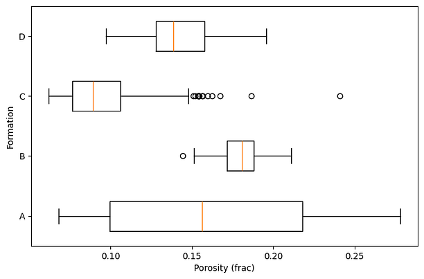
If we look at formation A, it shows a wide box across the whole porosity range, its median sits in the middle, and nothing about it suggests anything unusual. As we will see shortly, the median is sitting in the empty gap between two populations in the bimodal distribution, where almost no data actually sits.
Building the Raincloud Plot
Layer one: the cloud
The cloud layer is a half-violin plot. This is kernel density estimate drawn on one side only. We compute the density with gaussian_kde, scale it to a fixed height so every formation is comparable, and fill it in above the formation’s baseline.
def add_cloud(ax, values, ypos, width=0.35, colour=”#4C72B0”):
    kde = gaussian_kde(values)
    xs = np.linspace(values.min(), values.max(), 200)
    dens = kde(xs)
    dens = dens / dens.max() * width
    ax.fill_between(xs, ypos, ypos + dens, color=colour, alpha=0.5, linewidth=0)
Building xs between values.min() and values.max() clips the density to the actual range of the data, so the cloud can’t drift past your real readings the way a default violin does.
Dividing by dens.max() normalises every cloud to the same peak height, so you are comparing shapes rather than raw densities between each of the formations.
That normalisation has a cost worth knowing about: it makes an 18-point dataset can look as substantial as a 300-point dataset, which is exactly why the raw data goes in underneath. Drawing the cloud on one side keeps it compact and leaves room for those points.
Plotting all four formations:
fig, ax = plt.subplots(figsize=(8, 5))
for i, (vals, c) in enumerate(zip(groups, colours)):
    add_cloud(ax, vals, i, colour=c)
ax.set_yticks(range(len(formations)))
ax.set_yticklabels(formations)
ax.set_xlabel(”Porosity (frac)”)
plt.show()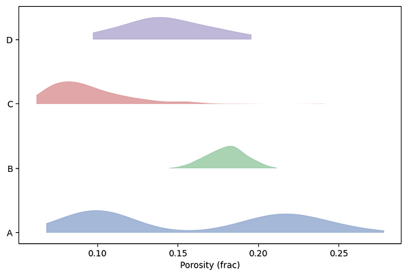
Formation A now shows its two humps plainly, which represents our bimodal distribution, C shows its left skew, and B is the narrow spike you would expect from a tight distribution.
Whilst we can see the distributions of the data a density curve has its own problem: it is a smooth estimate, and with few points it will invent a smoothness the data can’t support.
This is why we need to add the actual data points.
Layer two: the rain
The rain is the raw observations, scattered below the cloud with a little vertical jitter so points do not pile up and hide each other.
The jitter is purely cosmetic on the vertical axis and carries no meaning. The horizontal position is the real value.
Adding the rain under each cloud can be done using the following function
def add_rain(ax, values, ypos, spread=0.12, gap=0.06, colour=”#4C72B0”):
    jitter = rng.uniform(0, spread, size=len(values))
    ax.scatter(values, ypos - gap - jitter, s=8, color=colour, alpha=0.5,
               edgecolor=”none”)
and then recreating the plot:
fig, ax = plt.subplots(figsize=(8, 5))
for i, (vals, c) in enumerate(zip(groups, colours)):
    add_cloud(ax, vals, i, colour=c)
    add_rain(ax, vals, i, colour=c)
ax.set_yticks(range(len(formations)))
ax.set_yticklabels(formations)
ax.set_xlabel(”Porosity (frac)”)
plt.show()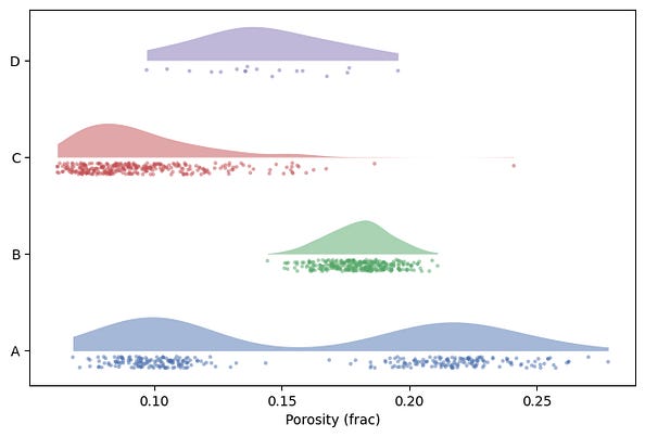
Formation D shows a smooth, reasonable distribution, but the rain shows only a handful of points. This smoothness was a result of the KDE filling in gaps .
The rain layer shows the real observations, how they are distributed and how many of them there are.
Layer three: the box
The summary generated by the boxplot is still worth keeping and can be added a thin horizontal box between the cloud and the rain.
The trick with matplotlib is setting manage_ticks=False, which stops the boxplot from resetting the y axis we have carefully set up.
def add_box(ax, values, ypos):
    ax.boxplot([values], positions=[ypos], vert=False, widths=0.08,
               manage_ticks=False, showfliers=False,
               medianprops=dict(color=”black”))
With all three layers in place we can generate the final plot:
fig, ax = plt.subplots(figsize=(8, 5))
for i, (vals, c) in enumerate(zip(groups, colours)):
    add_cloud(ax, vals, i, colour=c)
    add_box(ax, vals, i)
    add_rain(ax, vals, i, colour=c)
ax.set_yticks(range(len(formations)))
ax.set_yticklabels(formations)
ax.set_xlabel(”Porosity (frac)”)
ax.set_ylabel(”Formation”)
ax.set_ylim(-0.4, len(formations) - 0.3)
plt.show()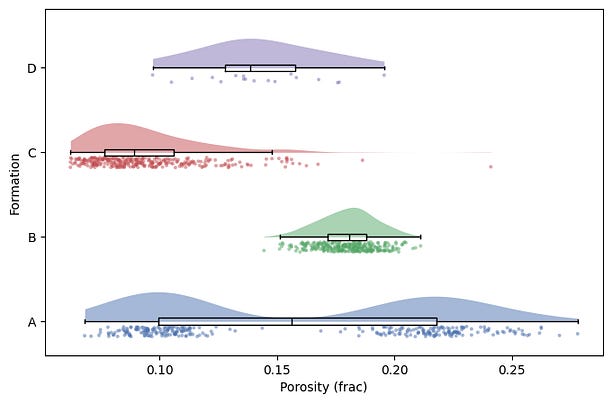
For each formation we can now see the shape, the raw data, and the summary at once, and you can check them against each other.
Formation A’s whiskers still span the whole range, but now the bimodal distribution and the gap in data points between can be seen.
Formation D’s tidy little box sits over a handful of points, so you know to discount it.
The chart makes the gap between summary and data visible instead of hiding it.
The Shortcut to a Raincloud Plot
As mentioned at the start of the article, there is also a dedicated library called PtitPrince for generating this type of plot, which has different ways of displaying them. ptitprince (GitHub — pog87/PtitPrince: python version of raincloud · GitHub) wraps all of this into roughly one call:
import ptitprince as pt

pt.RainCloud(x=”formation”, y=”porosity”, data=data, orient=”h”)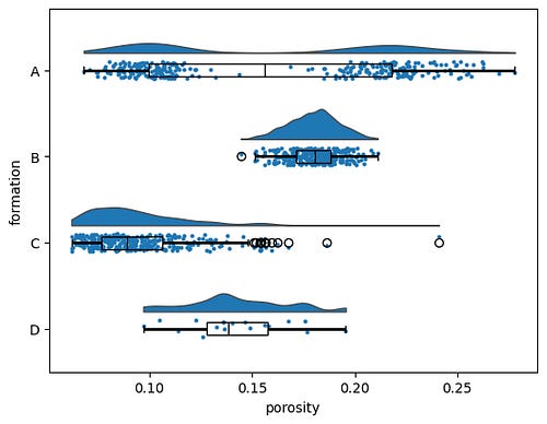
It is a fine option, though it has occasionally lagged behind newer seaborn and matplotlib versions, so check it works in your environment. The reason to keep the hand-built version is control: orientation, spacing, colour per group, how much jitter, whether the box shows outliers. Once the three helpers exist, you own all of that.
Where The Raincloud Plot Can Fall Over
The raincloud shouldn’t be seen as a default for every situation. Beyond a handful of groups it starts to get busy, because the eye has three elements per row to track, and a ridgeline plot reads more cleanly when you only care about shape across many groups. With well log data running to tens of thousands of samples, the rain turns into a solid smear and you have to thin it with transparency or subsampling, at which point it can mean less. And as formation D shows, with very few points the cloud is mostly interpolation, so trust the rain and treat the cloud as decoration.
Used in the right place, though, the plot can be a useful tool in the toolbox.
The density cloud is what makes a raincloud a raincloud, but it isn’t always worth the extra layer. Sometimes keeping the boxplot and overlaying just the raw points tells you everything you need, especially in exploratory work when you only want to check whether the summary is hiding something. I’ve written that simpler version up on Substack, building it in seaborn with group means and sample-size labels, along with where it starts to break down.
→ Boxplots Are Hiding Your Data. Here’s a Simple Fix
Reference: Allen M, Poggiali D, Whitaker K, Marshall TR, van Langen J, Kievit RA. Raincloud plots: a multi-platform tool for robust data visualization. Wellcome Open Research 2021, 4:63. https://wellcomeopenresearch.org/articles/4-63